Notes on GAN
2017-10-10
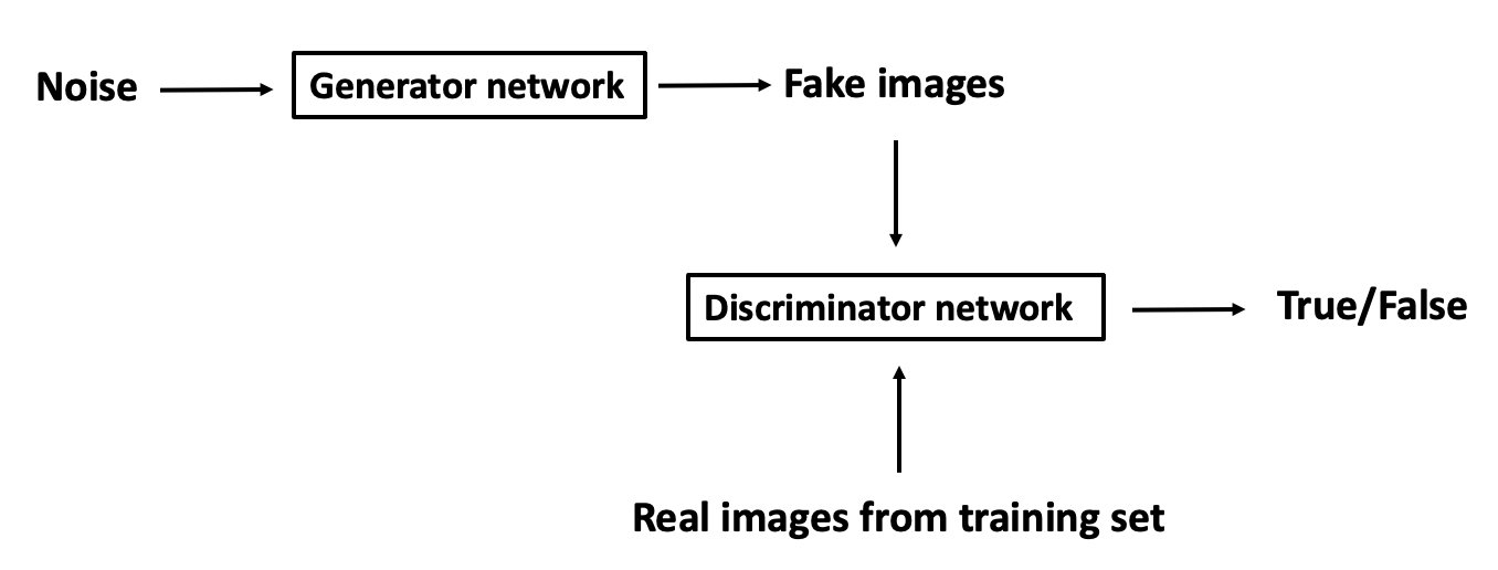
GAN (Generative Adversarial Network) is featured by two opponents: generator network and discriminator network. Generator network generates fake images from noise, trying to fool discriminator to classify them into real image, while discriminator trying to distinguish between real ones from the training set and fake images from generator.
1. Sketch of framework
2. Minimax of objective function
In the formula below, $\theta_d$ is discriminator’s parameter, while $\theta_g$ is generator’s parameter. $D_{\theta_d(\cdot)}$ is the output of discriminator which is a value between 0 and 1 meaning the likelihood of real image.
$$\min_{\substack{\theta_{g}}} \max_{\substack{\theta_{d}}} [E_{x \sim p_{data}(x)} logD_{\theta_d}(x) + E_{z \sim p_z(z)} log(1 - D_{\theta_{d}}(G_{\theta_{g}}(z))) ]$$
For discriminator, it wants to maximize the objective function so that $D_{\theta_d}(x)$ is close to 1 ($x$ is from real images) and $ D_{\theta_{d}}(G_{\theta_{g}}(z)))$ is close to zero ($G_{\theta_{g}}(z)$ is a generated fake image). On the contrary, generator wants to minimize objective such that $D_{\theta_{d}}(G_{\theta_{g}}(z)))$ is close to 1 (meaning discriminator is fooled into thinking $G(z)$ is real)
3. Algorithm
for #training iterations do
for k steps do
Sample minibatch of m noise samples {$z^{(1)}, ..., z^{(m)}$} from noise prior
Sample minibatch of m samples {$x^{(1)}, ..., x^{(m)}$} from data generating
distribution
Update the discriminator by ascending its stochastic gradient:
$$\nabla_{\theta_d} \frac{1}{m}\Sigma_{i=1}^{m} [logD(x^{(i)}) + log(1 - D(G(z^{(i)}))) ]$$
end for
Sample minibatch of m noise samples {$z^{(1)}, ..., z^{(m)}$} from noise prior $p_g(z)$
Update the generator by descending its stochastic gradient:
$$\nabla_{\theta_d} \frac{1}{m}\Sigma_{i=1}^{m} log(1 - D(G(z^{(i)})))$$
end for
4. Implementation Example: generate hand-written digits using Convolutional GAN
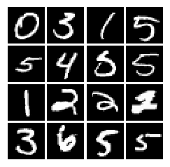
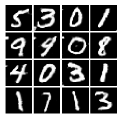
Here we use MNIST dataset which contains 60,000 training and 10,000 test images of human hand-written digits.
Sample images in MNIST dataset:
Original image dimension is $28 \times 28$, but is flattened by TensorFlow MNIST wrapper to a $784$d vector, i.e. dimension of input to network is (batch_size, $784$) where we use $128$ as batch_size in this example.
1. Discriminator: compute score for a batch of input images
Architecture |
|---|
| 32 Filters, 5x5, Stride 1, Leaky ReLU (alpha=0.01) |
| Max Pool 2x2, Stride 2 |
| 64 Filters, 5x5, Stride 1, Leaky ReLU (alpha=0.01) |
| Max Pool 2x2, Stride 2 |
| Fully Connected size 4 x 4 x 64, Leaky ReLU (alpha=0.01) |
| Fully Connected size 1 |
Code:
def discriminator(x):
    with tf.variable_scope("discriminator"):
        x_in = tf.reshape(x, [-1, 28, 28, 1])
        # Convolutional Layer #1
        conv1 =
          tf.layers.conv2d(inputs=x_in, filters=32, kernel_size=[5, 5], padding="valid", activation=leaky_relu)
        # Pooling Layer #1
        pool1 = tf.layers.max_pooling2d(inputs=conv1, pool_size=[2, 2], strides=2)
        # Convolutional Layer #2
        conv2 =
          tf.layers.conv2d(inputs=pool1, filters=64, kernel_size=[5, 5], padding="valid", activation=leaky_relu)
        # Pooling Layer #2
        pool2 = tf.layers.max_pooling2d(inputs=conv2, pool_size=[2, 2], strides=2)
        # flatten
        pool2_flat = tf.contrib.layers.flatten(pool2)
        # fully connected layer
        fc1 = tf.layers.dense(inputs=pool2_flat, units=1024, activation=leaky_relu)
        logits = tf.layers.dense(inputs=fc1, units=1)
        return logits
where the leaky RELU activation function is defined as
def leaky_relu(x, alpha=0.01):
    return tf.maximum(alpha*x, x)
2. Generator: generate images from a random noise vector.
Architecture |
|---|
| Fully connected of size 1024, ReLU |
| BatchNorm |
| Fully connected of size 7 x 7 x 128, ReLU |
| BatchNorm |
| Resize into Image Tensor |
| 64 conv2d^T (transpose) filters of 4x4, stride 2, ReLU |
| BatchNorm |
| 1 conv2d^T (transpose) filter of 4x4, stride 2, TanH |
Code:
def generator(z):
  with tf.variable_scope("generator"):
      fc1 = tf.layers.dense(inputs=z, units=1024, activation=tf.nn.relu)
      bn1 = tf.layers.batch_normalization(fc1)
      fc2 = tf.layers.dense(inputs=bn1, units=7*7*128, activation=tf.nn.relu)
      bn2 = tf.layers.batch_normalization(fc2)
      bn2_resized = tf.reshape(bn2, (-1, 7, 7, 128))
      convt1 = tf.contrib.layers.conv2d_transpose(bn2_resized, 64, (4,4), (2,2), activation_fn=tf.nn.relu)
      bn3 = tf.layers.batch_normalization(convt1)
      img = tf.contrib.layers.conv2d_transpose(bn3, 1, (4,4), (2,2), activation_fn=tf.nn.tanh)
      return img
3. Least squares loss function for GAN
Least squares loss is a newly proposed, more stable loss function than the original GAN’s.
$$l_G = \frac{1}{2}E_{z \sim p(z)}[D(G(Z))-1)^2]$$
$$l_D = \frac{1}{2}E_{x \sim p_{data}}[(D(X)-1)^2] + \frac{1}{2}E_{z \sim p(z)}[D(G(Z))^2]$$
Here we use average instead of computing the expectation.
Code:
def lsgan_loss(score_real, score_fake):
    G_loss = 0.5*tf.reduce_mean(tf.square(score_fake - 1))
    D_loss = 0.5*tf.reduce_mean(tf.square(score_real - 1))+0.5*tf.reduce_mean(tf.square(score_fake))
    return D_loss, G_loss
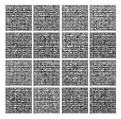
Result
First 200 iteration output:
1000 Iteration:
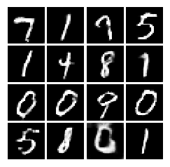
Final output:
References
- Goodfellow, Ian, et al. “Generative adversarial nets.” Advances in neural information processing systems. 2014.
- http://cs231n.stanford.edu/